The iris dataset is very widely used in the data science community, whether as a training aid, a tool for trying out new skills, or just a well-known set of numbers that can be used as background while demonstrating something in a blog. A relatively small dataset that displays some clear differences between three specieis of iris, it is clear why it has been popular.
Many people using iris will be unaware that it was first published in work by R A Fisher, a eugenicist with vile and harmful views on race. In fact, the iris dataset was originally published in the Annals of Eugenics. It is clear to me that knowingly using work that was itself used in pursuit of racist ideals is totally unacceptable.
Therefore, in this post, I highlight several alternatives. There are so many datasets freely available that this is a tiny start, and you can also use links I provide to explore further data repositories. But please investigate the data you use; iris shows us how seemingly innocuous data could have origins that should see it rejected.
Four alternative datasets
Penguins
Let’s start with the lovely penguins dataset. This is data about penguins collected by Dr. Kristen Gorman and the Palmer Station in Antarctica.
Allison Horst put it into a package, and her tweet about it was what first led me to learn about the history of the iris dataset.
🐧🐧🐧
— Allison Horst (@allison_horst) June 8, 2020
This penguin data is a great alternative to iris & available for use by CC0 🤩 Thank you Dr. Kristen Gorman w/ @UAFcfos, Marty Downs w/ @USLTER, & @PalmerLTER for help, info & making it available for use 🎉
Data, examples, & use info here: https://t.co/dSIqWNFlVw 🧵 1/6 pic.twitter.com/2Eu4AxoeZl
There are 344 cases and 7 columns. With both numerical and categorical variables, there are options for exploring, including looking for differentiators between the three species of penguin.
You can install the package using remotes::install_github("allisonhorst/palmerpenguins"). The dataset can then be accessed through the name penguins.
library(palmerpenguins)
str(penguins)
## tibble [344 x 7] (S3: tbl_df/tbl/data.frame)
##  $ species          : Factor w/ 3 levels "Adelie","Chinstrap",..: 1 1 1 1 1 1 1 1 1 1 ...
##  $ island           : Factor w/ 3 levels "Biscoe","Dream",..: 3 3 3 3 3 3 3 3 3 3 ...
##  $ bill_length_mm   : num [1:344] 39.1 39.5 40.3 NA 36.7 39.3 38.9 39.2 34.1 42 ...
##  $ bill_depth_mm    : num [1:344] 18.7 17.4 18 NA 19.3 20.6 17.8 19.6 18.1 20.2 ...
##  $ flipper_length_mm: int [1:344] 181 186 195 NA 193 190 181 195 193 190 ...
##  $ body_mass_g      : int [1:344] 3750 3800 3250 NA 3450 3650 3625 4675 3475 4250 ...
##  $ sex              : Factor w/ 2 levels "female","male": 2 1 1 NA 1 2 1 2 NA NA ...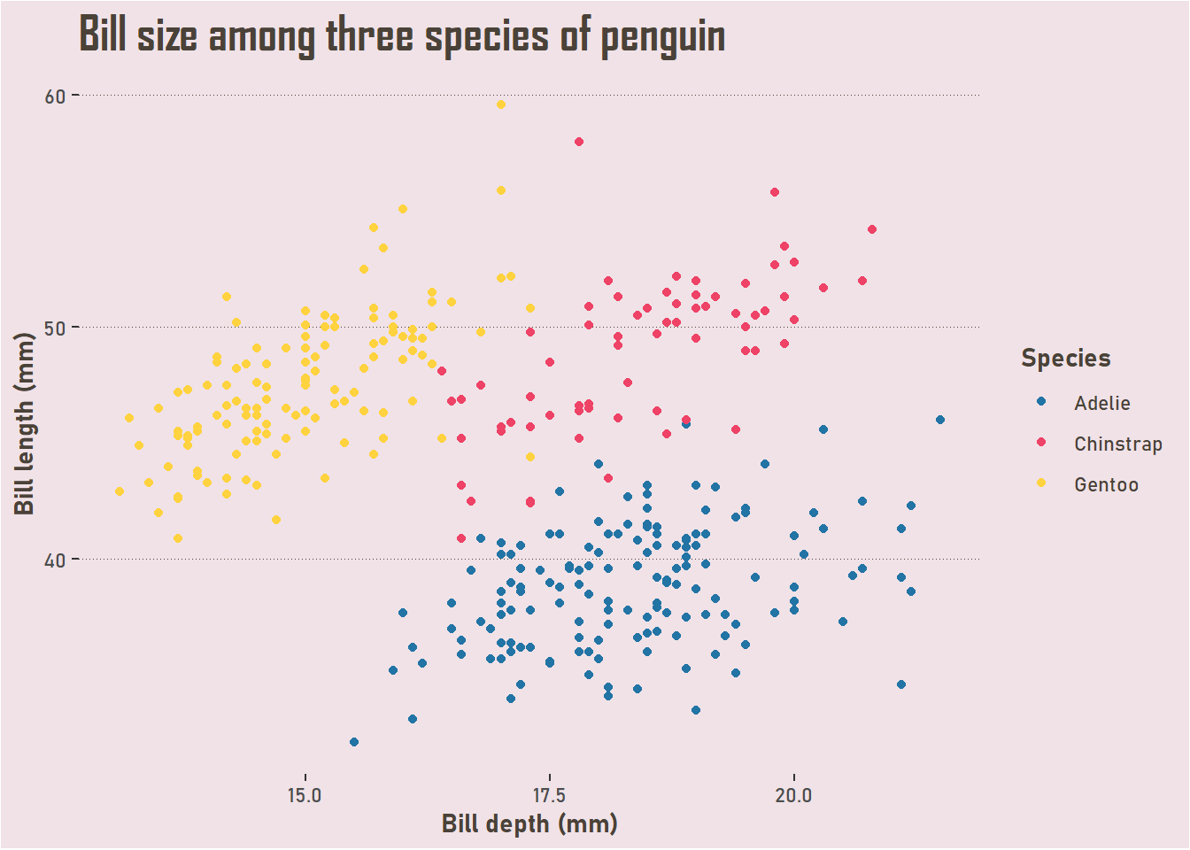
Hawks
Similarly, the hawks dataset is one I have been using in recent posts. This has 908 cases and 19 columns, though with some missing data there is also some practice to be had in preparing and cleaning your data! There are a number of measurements of three species of hawk. It was collected by students and faculty at Cornell College in Mount Vernon, Iowa.
The dataset can be found in the Stat2Data package.
library(Stat2Data)
data("Hawks")
str(Hawks)
## 'data.frame':    908 obs. of  19 variables:
##  $ Month       : int  9 9 9 9 9 9 9 9 9 9 ...
##  $ Day         : int  19 22 23 23 27 28 28 29 29 30 ...
##  $ Year        : int  1992 1992 1992 1992 1992 1992 1992 1992 1992 1992 ...
##  $ CaptureTime : Factor w/ 308 levels " ","1:15","1:31",..: 181 25 138 42 62 71 181 88 261 192 ...
##  $ ReleaseTime : Factor w/ 60 levels ""," ","10:20",..: 1 2 2 2 2 2 2 2 2 2 ...
##  $ BandNumber  : Factor w/ 907 levels " ","1142-09240",..: 856 857 858 809 437 280 859 860 861 281 ...
##  $ Species     : Factor w/ 3 levels "CH","RT","SS": 2 2 2 1 3 2 2 2 2 2 ...
##  $ Age         : Factor w/ 2 levels "A","I": 2 2 2 2 2 2 2 1 1 2 ...
##  $ Sex         : Factor w/ 3 levels "","F","M": 1 1 1 2 2 1 1 1 1 1 ...
##  $ Wing        : num  385 376 381 265 205 412 370 375 412 405 ...
##  $ Weight      : int  920 930 990 470 170 1090 960 855 1210 1120 ...
##  $ Culmen      : num  25.7 NA 26.7 18.7 12.5 28.5 25.3 27.2 29.3 26 ...
##  $ Hallux      : num  30.1 NA 31.3 23.5 14.3 32.2 30.1 30 31.3 30.2 ...
##  $ Tail        : int  219 221 235 220 157 230 212 243 210 238 ...
##  $ StandardTail: int  NA NA NA NA NA NA NA NA NA NA ...
##  $ Tarsus      : num  NA NA NA NA NA NA NA NA NA NA ...
##  $ WingPitFat  : int  NA NA NA NA NA NA NA NA NA NA ...
##  $ KeelFat     : num  NA NA NA NA NA NA NA NA NA NA ...
##  $ Crop        : num  NA NA NA NA NA NA NA NA NA NA ...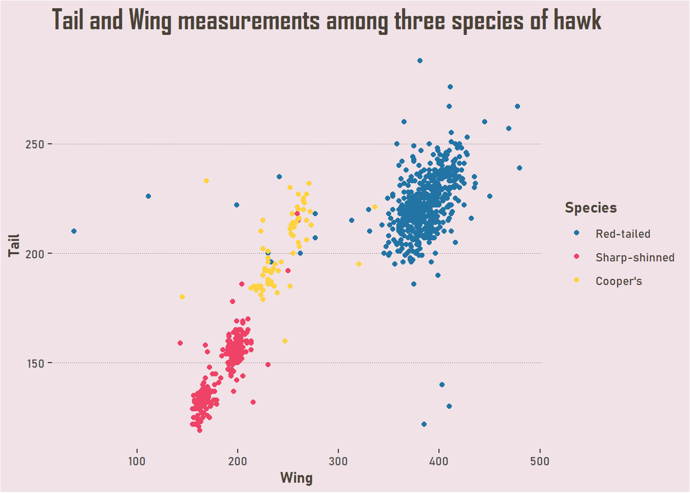
Mushrooms
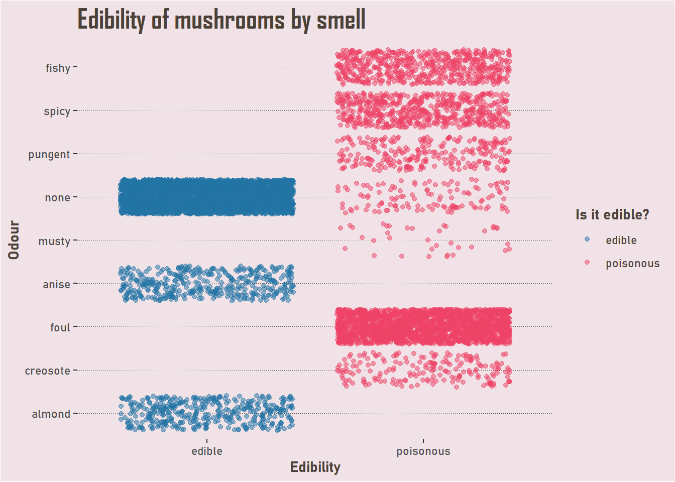
Another interesting dataset was drawn from The Audubon Society Field Guide to North American Mushrooms. It categorises mushrooms by a whole host of features, including details of the cap, gill, stalk and rings. It also records if they are edible or poisonous. This combination means there is a lot you can do, with 22 attributes to use as part of a classification task. And there are 8,124 cases!
You can download the csv from Kaggle, and although the original dataset is full of abbreviations, there is a key there, or you can use this case study in Machine Learning with R by François de Ryckel and copy the data cleaning steps, which I did to create this chart.
Cars
Perhaps what you really want in a replacement for iris is minimum set up - you don’t want to install a package you don’t use for anything else. Well, in that case, you might as well used mpg from ggplot2. I think it’s a little overused (as with iris, and many datasets available through popular packages), but it has a number of different categories, which is useful if you are getting started with data exploration.
The larger original dataset was first used by Ross Quinlan in ‘Combining Instance-Based and Model-Based Learning’ during the Tenth International Conference of Machine Learning.
library(ggplot2)
str(mpg)
## tibble [234 x 11] (S3: tbl_df/tbl/data.frame)
##  $ manufacturer: chr [1:234] "audi" "audi" "audi" "audi" ...
##  $ model       : chr [1:234] "a4" "a4" "a4" "a4" ...
##  $ displ       : num [1:234] 1.8 1.8 2 2 2.8 2.8 3.1 1.8 1.8 2 ...
##  $ year        : int [1:234] 1999 1999 2008 2008 1999 1999 2008 1999 1999 2008 ...
##  $ cyl         : int [1:234] 4 4 4 4 6 6 6 4 4 4 ...
##  $ trans       : chr [1:234] "auto(l5)" "manual(m5)" "manual(m6)" "auto(av)" ...
##  $ drv         : chr [1:234] "f" "f" "f" "f" ...
##  $ cty         : int [1:234] 18 21 20 21 16 18 18 18 16 20 ...
##  $ hwy         : int [1:234] 29 29 31 30 26 26 27 26 25 28 ...
##  $ fl          : chr [1:234] "p" "p" "p" "p" ...
##  $ class       : chr [1:234] "compact" "compact" "compact" "compact" ...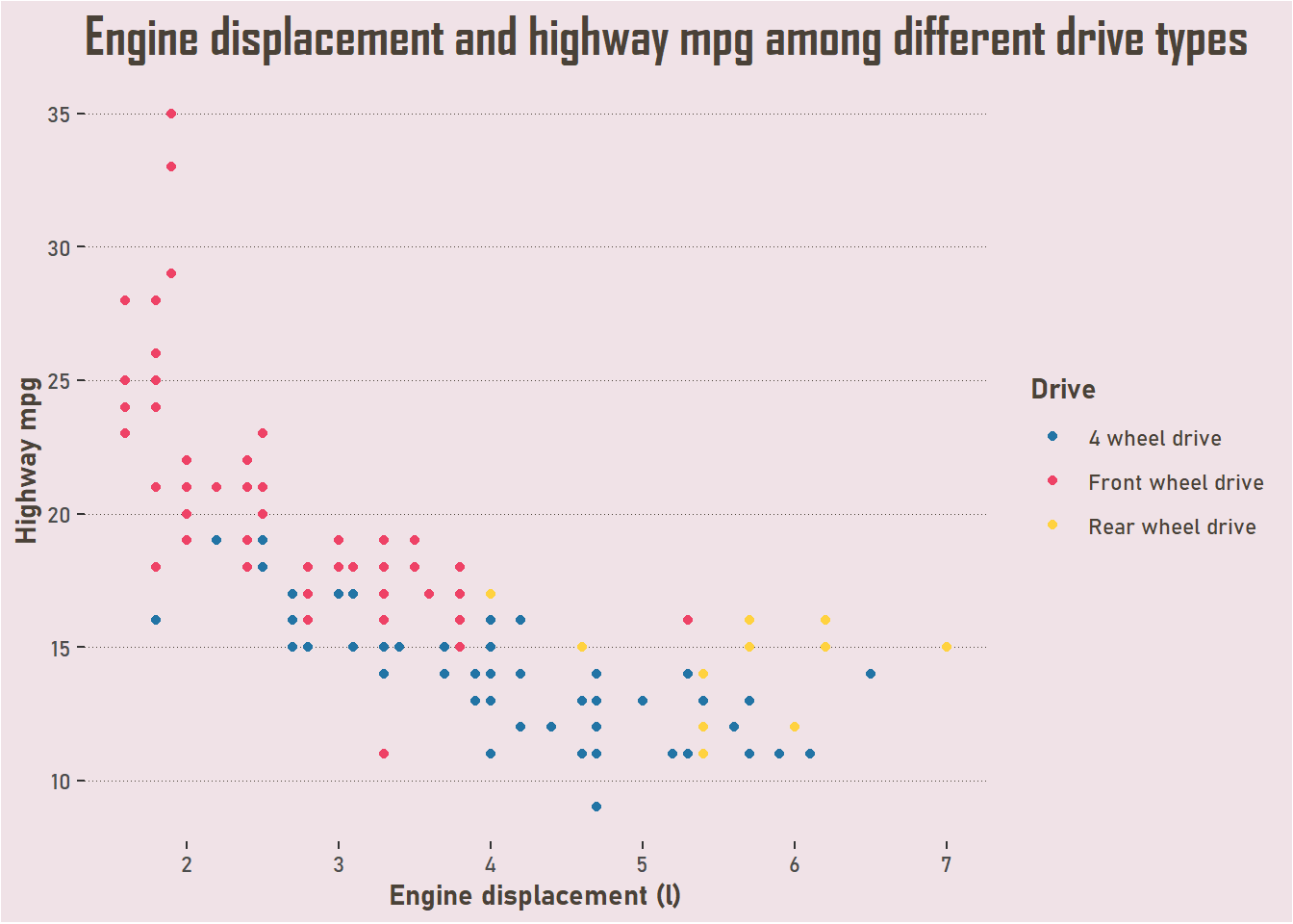
Four places to find data
Those datasets might not be quite right for you - or perhaps you want to avoid using the same data as everyone else. Well, here are some suggestions for places to look for data that will suit your needs.
RDataSets. This page provides a very helpful table of datasets available through R packages. You can see the number of rows, the number of columns, and also how many columns are binary or character (and therefore get a sense of what you might be able to do with them). Example datasets: Leaf shape; Airline passenger numbers; Air quality measures
The Tidy Tuesday repo. Every week, a new dataset is released to use, with instructions for how to access it in R. Going since 2018, there are now over 100 datasets available. They have plenty to explore, and you can find lots of examples of other people’s work. Example datasets: Passwords; Incarceration Trends; NYC Squirrel Census
UK government data. Open data published by the UK government - there are similar websites for many countries. I have frequently worked with government data and there is a lot to find out. Example datasets: Arrest statitistics; Qualifications; Government Spending
The Humanitarian Data Exchange. With over 19,000 datasets available, this is a great place to find data that can be used for social good. It can be filtered to find data relating to a country or region. Example datasets: Coronavirus cases; Earthquakes; Migration
Always make sure you know the provenance of the data you are using. And if you can, use your time working with meaningful datasets that expand your understanding of the world, and even help you to find things out that will allow you to agitate for a better society.