In May, I delivered a few training sessions for R beginners and I’m using those materials for some posts here. Following on from my two posts on ggplot2, this is based on my session of data.table, which could be my favourite R package. I actually wrote a post about why I like it so much here, but that doesn’t go into much detail of how to actually use it. In this post, rather than telling you everything I can think of at a high level, I’m just going to demonstrate how I might explore some data with data.table, and explain as I go along.
Having said that…I’ll lay out a few things upfront so they make more sense as we go through! These things are in my original post too but I’ll include here to make things easier.
First things first
The meaning of data.table
Although people talk about data tables to broadly apply to data structures with columns and rows, there are a few more specific definitions when we talk about data.table. It is a package in R that has been around for years and is well-maintained. That package enables you to create specific objects called data.tables. It also provides a specific way of working with those objects that is distinct from how you might be used to working with data in R.
The syntax
In this post, there will be many examples of using data.table code, but it’s worth understanding upfront that an awful lot of stuff you do with data.table is performed in three places. I’m going to repost this image from a wiki provided by the creators of data.table.
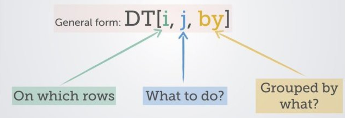
Here, DT is the name of your data.table object, which is followed by square brackets. Within those square brackets, you are referencing the following:
i: The first section is where you specify the rows that you want considered. It’s a place to filter or subset.
j: Stuff that’s going on in columns - you might be making a new one or modifying an existing one, for example. Generally where the action is happening.
by: Doing stuff by group - which is ridiculously handy to be able to do within this same line of code.
OK, that’s all we’re going to start with - let’s just dive in now.
The package in action
Let’s look at the hawks dataset we used for the ggplot2 posts - you might also remember I talked about this in my most recent post about not using the Iris dataset.
With the data.table library, we could use fread() to read in the csv, which will be quick and give us a data.table object. Lots of people who aren’t normally data.table users will still use fread() and fwrite() for reading in and writing out csvs because it is so speedy. In this example, I’m also selecting certain columns to keep, because the original data has a lot of columns.
library(data.table)

hawks <- fread('https://vincentarelbundock.github.io/Rdatasets/csv/Stat2Data/Hawks.csv',
               select = c('Species', 'Age', 'Sex', 'Wing', 'Weight', 'Tail', 'KeelFat', 'Tarsus', 'Year'))
However, this dataset is available through the package Stat2Data so it probably makes more sense to load it from there and convert to a data.table object.
library(data.table)
library(Stat2Data)

data("Hawks")
hawks <- as.data.table(Hawks)
colnames(hawks)
## [1] "Month" "Day" "Year" "CaptureTime" "ReleaseTime"
## [6] "BandNumber" "Species" "Age" "Sex" "Wing"
## [11] "Weight" "Culmen" "Hallux" "Tail" "StandardTail"
## [16] "Tarsus" "WingPitFat" "KeelFat" "Crop"Dropping columns
Because we imported the data from the package, it still has all the columns we don’t want. We can remove columns we don’t want by name:
hawks[, Month := NULL]
colnames(hawks)
## [1] "Day" "Year" "CaptureTime" "ReleaseTime" "BandNumber"
## [6] "Species" "Age" "Sex" "Wing" "Weight"
## [11] "Culmen" "Hallux" "Tail" "StandardTail" "Tarsus"
## [16] "WingPitFat" "KeelFat" "Crop"Welcome to the walrus operator! That’s the := you see there. This combination of characters is how to create or modify a column without needing to create a copy of the dataset. This is one of the magical elements of data.table. The things to notice in the above line are:
- The action is happening in the second section, j, where stuff relating to columns happens.
- Nothing got explictly assigned or reassigned - we didn’t need to use
<-- but the data.table has still updated to drop the column.
If we want to drop multiple rows, we can still modify in place but we need to pass a vector of the column names through:
hawks[, c("Day", "CaptureTime", "ReleaseTime") := NULL]
colnames(hawks)
## [1] "Year" "BandNumber" "Species" "Age" "Sex"
## [6] "Wing" "Weight" "Culmen" "Hallux" "Tail"
## [11] "StandardTail" "Tarsus" "WingPitFat" "KeelFat" "Crop"Another option is to name the columns we want to keep. As long as j returns a list, each element of the list will become a column in the resulting data.table. If you only want certain columns in your data.table, you can achieve this using a list, which in its short version is .(). Because there are more columns we want to drop than keep, this would make sense for us here.
hawks <- hawks[, .(Species, Age, Sex, Wing, Weight, Tail, KeelFat, Tarsus, Year)]

# View the first five rows
hawks[1:5]
## Species Age Sex Wing Weight Tail KeelFat Tarsus Year
## 1: RT I 385 920 219 NA NA 1992
## 2: RT I 376 930 221 NA NA 1992
## 3: RT I 381 990 235 NA NA 1992
## 4: CH I F 265 470 220 NA NA 1992
## 5: SS I F 205 170 157 NA NA 1992Be aware that we need to reassign our data.table with <- to save it here because we we aren’t using :=. Also, you can see that the columns have been reordered to match the order in the list we fed in, so you can use that trick if you want to rearrange your data.
New columns
While we’re thinking about :=, that’s also the way to add new columns without needing to reassign your dataset. Let’s say we want a column for indicating if a bird is above 1000 in Weight.
hawks[, Over1000Weight := Weight > 1000]
hawks[, .(Weight, Over1000Weight)]
## Weight Over1000Weight
## 1: 920 FALSE
## 2: 930 FALSE
## 3: 990 FALSE
## 4: 470 FALSE
## 5: 170 FALSE
## ---
## 904: 1525 TRUE
## 905: 175 FALSE
## 906: 790 FALSE
## 907: 860 FALSE
## 908: 1290 TRUEWe can look at the relevant columns to check them with a list, just like we did when naming columns to keep. Because we aren’t reassigning it, the result shows up as an output in the console rather than overwriting the data.table. However, the new column will be in the existing data.table because we assigned with :=.
colnames(hawks)## [1] "Species" "Age" "Sex" "Wing"
## [5] "Weight" "Tail" "KeelFat" "Tarsus"
## [9] "Year" "Over1000Weight"Missing data
There are a few ways to look for missing data. We can use the base function is.na() when filtering by rows, like this:
hawks[is.na(Weight)]## Species Age Sex Wing Weight Tail KeelFat Tarsus Year Over1000Weight
## 1: RT A 393 NA 238 NA NA 1992 NA
## 2: RT I 326 NA 215 NA NA 1993 NA
## 3: SS A F 194 NA 154 NA NA 1993 NA
## 4: SS I F 202 NA 164 NA NA 1995 NA
## 5: SS I M 162 NA 130 1 NA 1997 NA
## 6: RT I 361 NA 214 NA NA 1998 NA
## 7: RT I 271 NA 235 2 NA 1999 NA
## 8: SS I F 205 NA 161 NA NA 1999 NA
## 9: SS I F 190 NA 153 2 NA 2000 NA
## 10: RT A 406 NA 222 2 NA 2000 NAThis shows us rows where Weight has an NA value. We are performing this action in the first section within the square brackets, known as i, which is where actions relating to rows take place.
You can do this across all columns with complete.cases(), which is from the base stats package, negating it with a ! to find incomplete cases:
hawks[!complete.cases(hawks)]## Species Age Sex Wing Weight Tail KeelFat Tarsus Year Over1000Weight
## 1: RT I 385 920 219 NA NA 1992 FALSE
## 2: RT I 376 930 221 NA NA 1992 FALSE
## 3: RT I 381 990 235 NA NA 1992 FALSE
## 4: CH I F 265 470 220 NA NA 1992 FALSE
## 5: SS I F 205 170 157 NA NA 1992 FALSE
## ---
## 830: RT I 380 1525 224 3 NA 2003 TRUE
## 831: SS I F 190 175 150 4 NA 2003 FALSE
## 832: RT I 360 790 211 2 NA 2003 FALSE
## 833: RT I 369 860 207 2 NA 2003 FALSE
## 834: RT A 199 1290 222 1 NA 2003 TRUEOK, there are a LOT of incomplete cases. Looking at the data it seems likely that KeelFat and Tarsus are full of missing data. We can do this using the special built-in variable .N, which returns the number of observations in a group - or basically a way to count rows. Here we count the number of rows that are NA for these columns.
hawks[is.na(KeelFat), .N]## [1] 341hawks[is.na(Tarsus), .N]## [1] 833We might decide for our analysis we don’t want to include those variables if they are that incomplete, just like we dropped columns before.
hawks[, c("KeelFat", "Tarsus") := NULL]

# No need to reassign
hawks[1:5]
## Species Age Sex Wing Weight Tail Year Over1000Weight
## 1: RT I 385 920 219 1992 FALSE
## 2: RT I 376 930 221 1992 FALSE
## 3: RT I 381 990 235 1992 FALSE
## 4: CH I F 265 470 220 1992 FALSE
## 5: SS I F 205 170 157 1992 FALSELet’s review the incomplete cases again.
hawks[!complete.cases(hawks)]## Species Age Sex Wing Weight Tail Year Over1000Weight
## 1: RT A 393 NA 238 1992 NA
## 2: RT I 326 NA 215 1993 NA
## 3: SS A F 194 NA 154 1993 NA
## 4: SS I F 202 NA 164 1995 NA
## 5: CH A NA 480 198 1995 FALSE
## 6: SS I M 162 NA 130 1997 NA
## 7: RT I 361 NA 214 1998 NA
## 8: RT I 271 NA 235 1999 NA
## 9: SS I F 205 NA 161 1999 NA
## 10: SS I F 190 NA 153 2000 NA
## 11: RT A 406 NA 222 2000 NAWe could probably get rid of those; there are now only 11 out of 908 observations. This is just a case of assigning the output from our complete.cases() line to the name of our dataset.
hawks <- hawks[complete.cases(hawks)]
hawks[is.na(Weight)]
## Empty data.table (0 rows and 8 cols): Species,Age,Sex,Wing,Weight,Tail...But the very observant will have noticed that there is also missing data in some of the columns that doesn’t seem to be registering. For example, the first row of the dataset isn’t in this summary of incomplete cases, even though it’s missing information on sex.
hawks[1]## Species Age Sex Wing Weight Tail Year Over1000Weight
## 1: RT I 385 920 219 1992 FALSEThat’s because the Sex variable isn’t an NA value; it appears to just be an empty string. Let’s check that by looking at the unique values for Sex. We’re looking at a column so working in the second section of the square brackets, after a comma to give space for the first section.
hawks[, unique(Sex)]## [1] F M
## Levels: F MAs suspected, it’s an empty string rather than an NA value. But how many are there? We can use the useful .N, but also use our third section, by, to get results for each different value in the Sex column. So we have nothing in the first section (because we aren’t doing anything with rows), .N in the second section, and Sex in the third section.
hawks[, .N, by = Sex]## Sex N
## 1: 570
## 2: F 170
## 3: M 157Oh dear - hawks with unknown sex make up most of the dataset, so we can’t really just remove them. For now, we’ll make it a bit more explicit the data is unknown. Here we are using := so we don’t have to reassign the data.table object. We’re also filtering the rows this applies to in the i section so it only changes the value where the Sex value is an empty string.
hawks[Sex == "", Sex := "Unknown"]
hawks[1:5]
## Species Age Sex Wing Weight Tail Year Over1000Weight
## 1: RT I Unknown 385 920 219 1992 FALSE
## 2: RT I Unknown 376 930 221 1992 FALSE
## 3: RT I Unknown 381 990 235 1992 FALSE
## 4: CH I F 265 470 220 1992 FALSE
## 5: SS I F 205 170 157 1992 FALSEWe should check the other character columns.
hawks[, .N, by = Species]## Species N
## 1: RT 572
## 2: CH 69
## 3: SS 256hawks[, .N, by = Age]## Age N
## 1: I 677
## 2: A 220Great, both Species and Age are complete columns.
Changing category values
We saw above how we could change a value by filtering it first. Let’s do that for the other sex values.
hawks[Sex == "F", Sex := "Female"]
hawks[Sex == "M", Sex := "Male"]
We can then change this to a factor variable, to ensure only these values can be used. While factor() isn’t a function specific to data.table, it works nicely within the syntax.
hawks[, Sex := factor(Sex, levels = c("Female", "Male", "Unknown"))]
levels(hawks[, Sex])
## [1] "Female" "Male" "Unknown"And the same for Species, but this time redefining the values after they’ve become factors so you see both ways.
hawks[, Species := factor(Species, levels = c("CH", "RT", "SS"))]
levels(hawks$Species) <- c("Cooper's", "Red-tailed", "Sharp-shinned")

levels(hawks[, Species])
## [1] "Cooper's" "Red-tailed" "Sharp-shinned"Exploring the data
So far we’ve been looking at the data for issues that we want to clean up, but you can use data.table to answer questions you have about the data too. Here’s an example to find out which species had the most adults recorded in the year 2000.
The first step is to filter the data to the year 2000 (in the i section), and count the rows (in the j section) while grouping the data by Species and Age (in the by section - see how we can group by multiple variables). We could just use .N in the second section, but by enclosing it in a list like that, we can also name the column, which gives us more power over the output.
# Filter by year, then count cases while grouping by species and age
age_species_2000 <- hawks[Year == 2000, .(Count = .N), by = .(Species, Age)]
age_species_2000
## Species Age Count
## 1: Sharp-shinned I 12
## 2: Red-tailed I 62
## 3: Red-tailed A 17
## 4: Cooper's A 4
## 5: Sharp-shinned A 16
## 6: Cooper's I 4OK, but actually we are only interested in Adults so let’s filter again.
# Filter to adults
adult_species_2000 <- age_species_2000[Age == "A"]
adult_species_2000
## Species Age Count
## 1: Red-tailed A 17
## 2: Cooper's A 4
## 3: Sharp-shinned A 16Obviously we can see by looking at the table what the answer is, but if we want the output as a value, there are some more steps. We order using order() in the i section, with a minus before the column name to show we want the results descending.
# Order by count
ordered <- adult_species_2000[order(-Count)]
ordered
## Species Age Count
## 1: Red-tailed A 17
## 2: Sharp-shinned A 16
## 3: Cooper's A 4Finally, we can get the value by specifying we want the first row only, and the value for Species - because this is not in a list, it will be returned as a value rather than a one row, one column data.table
# Select the value for the species in the first row
most_adults <- ordered[1, Species]
most_adults
## [1] Red-tailed
## Levels: Cooper's Red-tailed Sharp-shinnedIf you wanted, you could chain this all together with back to back square brackets!
hawks[Year == 2000, .(Count = .N), by = .(Species, Age)][Age == "A"][order(-Count)][1, Species]## [1] Red-tailed
## Levels: Cooper's Red-tailed Sharp-shinnedThe power of data.table
Here, we’ve covered:
Reading in data
Adding columns
Dropping columns
Rearranging columns
Renaming columns
Looking for missing data
Counting rows / observations
Filtering rows based on conditions
Grouping by one or multiple variables
Returning values rather than full datasets
There are loads more things you can do with data.table, and the data.table objects are flexible enough to be used with lots of other packages. This is just a speedy exploration of some stuff that I need to do all the time! And speedy is the word - a big advantage of data.table is how fast it performs, particularly with large datasets.
I hope this helps you to get started with data.table and you enjoy finding out how useful it can be!