Last year, I wrote about the Iris dataset, which is used a lot in data science training and coding examples but was originally published in the Journal of Eugenics. I don’t want to use it now I am aware of that. However, there are a lot of resources that reference or use it, a lot of which would have been published before this fact was widely discussed. For example, I am part of a book group reading Hands-On Machine Learning, and my heart sank when we got to Chapter 4, where the Iris dataset is used to accompany discussion of logistic and softmax regression.
However, as my previous post on the subject made clear, there are alternatives to Iris! So rather than discuss the chapter as is, or skip it altogether, I pulled the relevant code from the available repo to see if I could alter it satisfactorily. I used the hawks dataset, which has come up in several of my previous posts; it’s good for classification problems because there are three distinct species of hawk in the data, with a number of features to help identify them.
Below is the updated code demonstrating these regression approaches. I have added comments where I have changed something from the original.
I did have to work through the code chunks to find out what I needed to change - although the most important change was reading in different data, I also needed to change some of the values on the charts so the sizing and labels worked, for example. But the key thing to know here is this took me about 5 minutes! It was really easy! It was definitely worth doing to mean I could show visual examples of how this stuff works.
I’d really encourage you to be thoughtful about the data you are using, even when a dataset is already provided. This showed me how simple it was.
import pandas as pd
import numpy as np
import matplotlib.pyplot as plt

# Read in hawks dataset instead of Iris
hawks = pd.read_csv('https://vincentarelbundock.github.io/Rdatasets/csv/Stat2Data/Hawks.csv')
# Remove a few cases with missing data
hawks = hawks[~hawks['Wing'].isnull()]

# Select feature to predict (y) and feature to use in making predictions (X)
X = hawks[['Wing']].to_numpy()  # wing length
RT = hawks['Species'] == "RT"
y = RT.astype(np.int).to_numpy()  # 1 if Red-Tailed, else 0

from sklearn.linear_model import LogisticRegression
log_reg = LogisticRegression(solver="lbfgs", random_state=42)
log_reg.fit(X, y)

# Changed the numbers to 150, 450 instead of 0, 3,
# to reflect the different range of values
# in the hawks dataset for X
X_new = np.linspace(150, 450, 1000).reshape(-1, 1)
y_proba = log_reg.predict_proba(X_new)

# Change labels
plt.plot(X_new, y_proba[:, 1], "g-", linewidth=2,
          label="Red-Tailed")
plt.plot(X_new, y_proba[:, 0], "b--", linewidth=2,
          label="Not Red-Tailed")

decision_boundary = X_new[y_proba[:, 1] >= 0.5][0]

plt.figure(figsize=(8, 3))
plt.plot(X[y==0], y[y==0], "bs")
plt.plot(X[y==1], y[y==1], "g^")
plt.plot([decision_boundary, decision_boundary], [-1, 2], "k:", linewidth=2)
# Change labels
plt.plot(X_new, y_proba[:, 1], "g-", linewidth=2,
        label="Red-Tailed")
plt.plot(X_new, y_proba[:, 0], "b--", linewidth=2,
        label="Not Red-Tailed")
plt.text(decision_boundary+0.02, 0.15, "Decision  boundary",
          fontsize=14, color="k", ha="center")
plt.arrow(decision_boundary, 0.08, -0.3, 0, head_width=0.05,
          head_length=0.1, fc='b', ec='b')
plt.arrow(decision_boundary, 0.92, 0.3, 0, head_width=0.05,
          head_length=0.1, fc='g', ec='g')
plt.xlabel("Wing length (cm)", fontsize=14) # Change label
plt.ylabel("Probability", fontsize=14)
plt.legend(loc="center left", fontsize=14)
plt.axis([150, 450, -0.02, 1.02]) # Change axis range
# save_fig("logistic_regression_plot") # Can save if required
plt.show()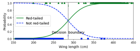
from sklearn.linear_model import LogisticRegression

X = hawks[['Wing', 'Tail']].to_numpy()   # tail length, wing length
y = RT.astype(np.int).to_numpy()

log_reg = LogisticRegression(solver="lbfgs", C=10**10, random_state=42)
log_reg.fit(X, y)

# Change numbers to reflect range of feature
x0, x1 = np.meshgrid(
        np.linspace(150, 450, 500).reshape(-1, 1),
        np.linspace(100, 300, 200).reshape(-1, 1),
    )
X_new = np.c_[x0.ravel(), x1.ravel()]

y_proba = log_reg.predict_proba(X_new)

plt.figure(figsize=(10, 4))
plt.plot(X[y==0, 0], X[y==0, 1], "bs")
plt.plot(X[y==1, 0], X[y==1, 1], "g^")

zz = y_proba[:, 1].reshape(x0.shape)
contour = plt.contour(x0, x1, zz, cmap=plt.cm.brg)


left_right = np.array([2.9, 7])
boundary = -(log_reg.coef_[0][0] * left_right + log_reg.intercept_[0]) / log_reg.coef_[0][1]

plt.clabel(contour, inline=1, fontsize=12)
plt.plot(left_right, boundary, "k--", linewidth=3)
plt.text(3.5, 1.5, "Not Red-Tailed", fontsize=14, color="b", ha="center") # Change label
plt.text(6.5, 2.3, "Red-Tailed", fontsize=14, color="g", ha="center") # Change label
plt.xlabel("Wing length", fontsize=14)
plt.ylabel("Tail width", fontsize=14)
plt.axis([100, 500, 100, 300]) # Change axes range
# save_fig("logistic_regression_contour_plot")
plt.show()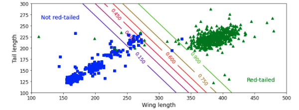
# For softmax regression, need to code species as numbers
hawks['Species_Category'] = hawks['Species'].astype('category')
hawks['Species_Category'] = hawks['Species_Category'].cat.codes
X = hawks[['Wing', 'Tail']].to_numpy() # Wing, Tail
y = hawks['Species_Category'].to_numpy() # Use new Species_Category field
softmax_reg = LogisticRegression(multi_class="multinomial",
solver="lbfgs", C=10, random_state=42)
softmax_reg.fit(X, y)
x0, x1 = np.meshgrid(
np.linspace(100, 500, 500).reshape(-1, 1), # sensible boundaries
np.linspace(100, 300, 200).reshape(-1, 1), # sensible boundaries
)
X_new = np.c_[x0.ravel(), x1.ravel()]
y_proba = softmax_reg.predict_proba(X_new)
y_predict = softmax_reg.predict(X_new)
zz1 = y_proba[:, 1].reshape(x0.shape)
zz = y_predict.reshape(x0.shape)
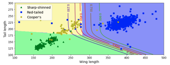
plt.figure(figsize=(10, 4))
plt.plot(X[y==2, 0], X[y==2, 1], "g^", label="Sharp-shinned")
plt.plot(X[y==1, 0], X[y==1, 1], "bs", label="Red-tailed")
plt.plot(X[y==0, 0], X[y==0, 1], "yo", label="Cooper's")
from matplotlib.colors import ListedColormap
custom_cmap = ListedColormap(['#fafab0','#9898ff','#a0faa0'])
plt.contourf(x0, x1, zz, cmap=custom_cmap)
contour = plt.contour(x0, x1, zz1, cmap=plt.cm.brg)
plt.clabel(contour, inline=1, fontsize=12)
plt.xlabel("Wing length", fontsize=14)
plt.ylabel("Tail length", fontsize=14)
plt.legend(loc="center left", fontsize=14)
plt.axis([100, 500, 100, 300])
# save_fig("softmax_regression_contour_plot")
plt.show()