Using {tidymodels} with the food tracker dataset

Mar 6, 2021 in PROJECT • R
r tidymodels model-selection resolution-tracker
5 min read

Using the data from my food tracker diary, I’m going to explore {tidymodels}, which offers a route into modelling and machine learning in the R ecosystem, curating relevant packages. I haven’t used it before so this is pretty new to me.

We’ve already done some feature engineering, but I’ll start by doing a few extra things to get the data into a more useful shape. All of the predictor columns here are boolean, so I’ll turn them into numeric columns so they are easier for the models to interpret. I’ll also reduce the dataset just to the columns I’m interested in using. Finally, I’m not really interested in whether the day is pescetarian or vegetarian specifically, so I’ll combine those categories so we can do binary classification: did I eat meat that day or not?

# Combine Pescetarian and Vegtarian categories
food_by_day[Diet == "P"|Diet == "V", Diet := "PV"]

# Reduce to relevant columns
food_by_day_clean <- food_by_day[, .(Date, Diet, 
                                     Monday, Tuesday, 
                                     Wednesday, Thursday, 
                                     Friday, Saturday, Sunday, 
                                     Weekend, FirstWeek, 
                                     LastWeek, Holiday)]

# Transform boolean to numeric
logical_cols <- names(Filter(is.logical, food_by_day_clean))
food_by_day_clean[,
                  (logical_cols):= lapply(.SD, as.numeric),
                  .SDcols = logical_cols]

I’ll want to split my data into test and training sets. I actually don’t have a lot of data - only 366 days in 2020 - so as my categories are imbalanced, I’m going to make sure I use stratified sampling to avoid having very few meat-eating days in the test set.

library(tidymodels)

set.seed(111) # Makes randomness reproducible

# Split the data into training and test sets
food_split <- initial_split(food_by_day_clean, 
                            prop = 3/4, 
                            strata = Diet) # Reflect balance in both sets

Then, the first step regardless of model is to create a ‘recipe’. There are actually a lot of things you can do in this step, including some of the feature engineering I’ve already done. Here, once I’ve set the recipe (i.e. formula), I update the Date column so it’s an ID column, and not used for prediction. I also use step_zv() to remove variables that contain only a single value, although I don’t think this is the case for any of mine. Finally, I’ve got step_corr() to deal with highly correlated variables. I know there’ll be some crossover in my features - after all I created all of them from the date! - so I want to guard against anything too extreme here.

food_recipe <- 
  recipe(Diet ~ ., data = food_by_day_clean) %>%
  update_role(Date, new_role = "Id") %>%
  step_zv(all_predictors())  %>%
  step_corr(all_predictors()) %>%
  prep()

Now it’s time to start training models! This time, we’ll look at Random Forest, Linear Regression and Support Vector Machines. I’ll go through Random Forest more slowly, then run the other two quickly after that.

Model training

We start off by defining the model and its engine, and then combine with the recipe in a workflow.

## RANDOM FOREST

rf_model <- 
  rand_forest() %>%
  set_engine("ranger") %>%
  set_mode("classification") 

rf_workflow <- workflow() %>%
  add_recipe(food_recipe) %>%
  add_model(rf_model)

You can test parameter ranges here, but to avoid an overly long post I’ll keep the workflow simple. It’s then just a case of applying the workflow to the data. You can just use the food_split dataset and it will know to use the training part for training.

rf_fit <- rf_workflow %>%
  last_fit(food_split)

Here are the same steps for the other models.

## LINEAR REGRESSION

lr_model <- 
  logistic_reg() %>%
  set_engine("glm") %>%
  set_mode("classification") 

lr_workflow <- workflow() %>%
  add_recipe(food_recipe) %>%
  add_model(lr_model)

lr_fit <- lr_workflow %>%
  last_fit(food_split)

## SVM

svm_model <- 
  svm_poly() %>%
  set_engine("kernlab") %>%
  set_mode("classification") 

svm_workflow <- workflow() %>%
  add_recipe(food_recipe) %>%
  add_model(svm_model)

svm_fit <- svm_workflow %>%
  last_fit(food_split)

Results

rf_performance <- rf_fit %>% collect_metrics()
rf_performance

## # A tibble: 2 x 4
##   .metric  .estimator .estimate .config             
##   <chr>    <chr>          <dbl> <chr>               
## 1 accuracy binary         0.615 Preprocessor1_Model1
## 2 roc_auc  binary         0.584 Preprocessor1_Model1

lr_performance <- lr_fit %>% collect_metrics()
lr_performance

## # A tibble: 2 x 4
##   .metric  .estimator .estimate .config             
##   <chr>    <chr>          <dbl> <chr>               
## 1 accuracy binary         0.648 Preprocessor1_Model1
## 2 roc_auc  binary         0.584 Preprocessor1_Model1

svm_performance <- svm_fit %>% collect_metrics()
svm_performance

## # A tibble: 2 x 4
##   .metric  .estimator .estimate .config             
##   <chr>    <chr>          <dbl> <chr>               
## 1 accuracy binary         0.626 Preprocessor1_Model1
## 2 roc_auc  binary         0.560 Preprocessor1_Model1

OK, so these are all…not incredible. Which probably isn’t a huge surprise - it’s a small dataset, with limited features, and I haven’t done much to tune the models! But looking at the scores, the logistic regression models has the highest accuracy and highest ROC AUC.

# Generate predictions from the test set
lr_predictions <- lr_fit %>% collect_predictions()

# Generate a confusion matrix
lr_predictions %>% 
  conf_mat(truth = Diet, estimate = .pred_class)

##           Truth
## Prediction  M PV
##         M   8  7
##         PV 25 51

Looking at a confusion matrix, things aren’t looking great. Of the days predicted to be meat-eating days, 8 were and 7 weren’t - it’s virtually a coin flip. On the other hand, most non meat-eating days were accurately predicted. With a lot of meat-eating days predicted to be non meat-eating days, it looks like this model is tending to plump for the more prevalant category. So if we were looking to refine this model, one key thing to do would be to balance the classes.

Bearing in mind this isn’t a great model, we don’t want to get too carried away with what it tells us, but you can look at the variable importance using the package vip.

library(vip)
lr_fit %>% 
  pluck(".workflow", 1) %>%   
  pull_workflow_fit() %>% 
  vip(num_features = 12)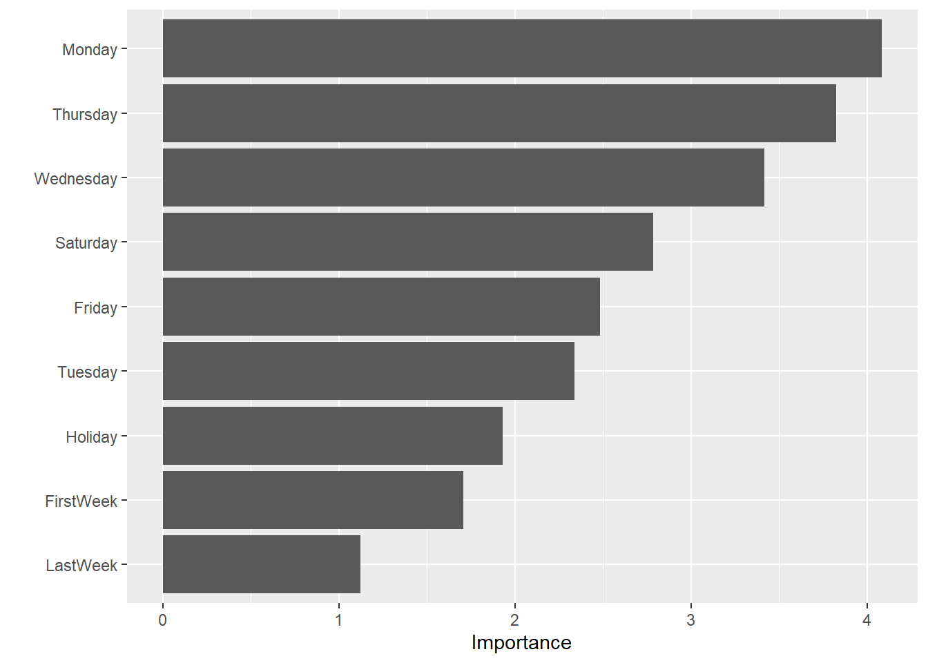

So this model indicates that Mondays are particularly important to the predictions it makes. Maybe I’m subconsciously doing meat-free Mondays!

Having explored {tidymodels} here, next time I might try to demonstrate the equivalent in Python, and see where that takes us.

Model training

Results

Other reading