I explored how often curators of @WeAreRLadies tweet in my last post. In this post, I go a little further with this analysis and explore how activity changes depending on the day of the week and time of day.
I’m using the same data that I retrieved using rtweet previously. I’m also going to use the same plot theme.
library(data.table)
library(ggplot2)
library(lubridate)
extrafont::loadfonts(device="win") #ensure fonts are loaded


rladies_tweets <- fread('rladies_tweets.csv')
rladies_tweets <- rladies_tweets[, .(created_at, status_id)]


plot_theme <- theme(
  plot.background = element_rect(fill = "#5FBFF9"),
  legend.background = element_rect(fill = "#5FBFF9"),
  legend.key=element_blank(),
  panel.background = element_rect(fill = "#5FBFF9"),
  text = element_text(colour = "#143642",
                      family = "Bahnschrift",
                      size = 18),
  title = element_text(face = "bold"),
  plot.title = element_text(family = "Agency FB",
                            size = 26),
  panel.grid.major.y = element_line(colour = "#143642",
                                    size = 0.2,
                                    linetype = "dotted"),
  panel.grid.major.x = element_blank(),
  panel.grid.minor = element_blank()
)

tweet_cols <- c("#D30C7B", "#EC9A29")
Firstly, I want to look at how activity changes depending on the day of the week. I need to create a column for weekday, which I can do by using the weekday() function on the column that contains the date and time of the tweet. I transform this column into an ordered factor so it will display in the correct order on graphs.
rladies_tweets[, created_at := as_datetime(created_at)]
# Add a column for weekday
rladies_tweets[, weekday := weekdays(created_at)]
weekday_levels <- c("Monday", "Tuesday", "Wednesday",
                    "Thursday", "Friday", "Saturday", "Sunday")
rladies_tweets[, weekday := factor(weekday, weekday_levels)]
# Add a column to group weeks by start date
rladies_tweets[, week_start := cut(created_at, "week")]
I then need to count the number of tweets each day of the week for each curation period. There is an additional step to consider here because I want to have rows indicating if there have been no tweets on a given day so this will be considered when calculating the range and median.
weekday_counts <- rladies_tweets[, .N, by = c("week_start", "weekday")]
# Ensure there is a row for every weekday/week start combo
setkeyv(weekday_counts, c("week_start", "weekday"))
weekday_counts <- weekday_counts[CJ(levels(rladies_tweets[, week_start]),
                                    unique(rladies_tweets[, weekday])), ]
# Change NA to 0
weekday_counts[is.na(N), N := 0]
However, I also want to remove rows that relate to weeks with no curator, which I’m defining as weeks with 1 or fewer tweets.
# Find low activity weeks
week_counts_info <- rladies_tweets[, .N, by = week_start]
no_curator = week_counts_info[N <= 1, as.character(week_start)]
# Remove weeks from data
weekday_counts <- weekday_counts[!week_start %in% no_curator]
Finally, using ggplot() we can see the activity by weekday.
ggplot(weekday_counts, aes(x = weekday, y = N)) +
  geom_boxplot(width = 0.5, fill = tweet_cols[2]) +
  plot_theme +
  labs(
    x = NULL, y = NULL,
    title = "Tweets from @WeAreRLadies",
    subtitle = "From 7 October 2019, excluding weeks with 0 or 1 tweets",
    caption = "\nSource: Data collected from Twitter's REST API via rtweet"
) 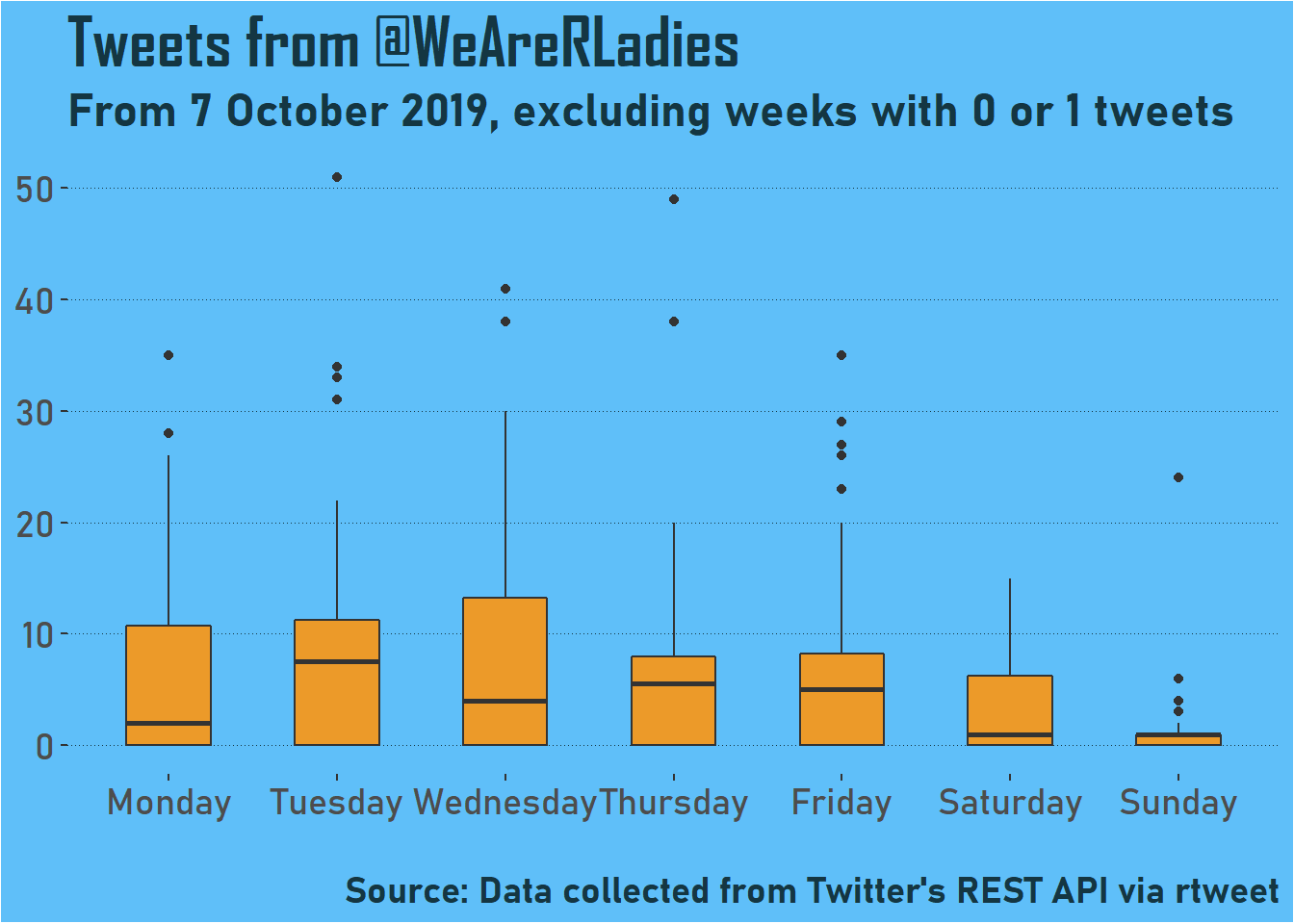
This shows pretty much what I’d expect. The lowest activity is on Sunday, which is the changeover day - technically as a curator you are in charge from Monday to Saturday. I would say that the IQR from Monday to Wednesday looks higher than Thursday to Saturday, with some curators perhaps frontloading their content. It’s also interesting to see the low medians on Monday (perhaps people are starting off the week with just a few introductory words) and Saturday (I imagine a lot of people view this as part of their normal work week).
Let’s look in a little more detail at timing. I want to make a tile plot showing number of tweets each hour of each weekday. This isn’t super compelling because the number of tweets might not always be high enough to draw really solid conclusions, but it’s a chart type I enjoy so let’s go for it!
Similarly to above, we need a dataset that has tweet counts for each hour of each weekday.
# Column for hour tweeted
rladies_tweets[, hour := hour(created_at)]

# Count by weekday and hour
time_counts <- rladies_tweets[, .N, by = c("weekday", "hour")]

# Ensure 0 tweets is shown
setkeyv(time_counts, c("weekday", "hour"))
time_counts <- time_counts[CJ(levels(rladies_tweets[, weekday]),
                              unique(rladies_tweets[, hour])),]
time_counts[is.na(N), N := 0]

# Order factor
time_counts[, weekday := factor(weekday, weekday_levels)]
We can use geom_tile() to plot this. The function coord_equal() gives us neat squares.
# Labels for time
time_labels = paste0(stringr::str_pad(seq(0, 23), 2, "left", 0), ":00")
ggplot(time_counts, aes(hour, forcats::fct_rev(weekday), fill = N)) +
geom_tile() +
plot_theme +
theme(axis.text.x = element_text(angle = 90)) +
scale_fill_gradient(low = tweet_cols[2], high = "red") +
scale_x_continuous(breaks = seq(0, 23), labels = time_labels) +
coord_equal() +
labs(
x = NULL, y = NULL,
title = "Tweets from @WeAreRLadies",
subtitle = "Year from 7 October 2019",
caption = "\nSource: Data collected from Twitter's REST API via rtweet",
fill = "Number\nof tweets"
) 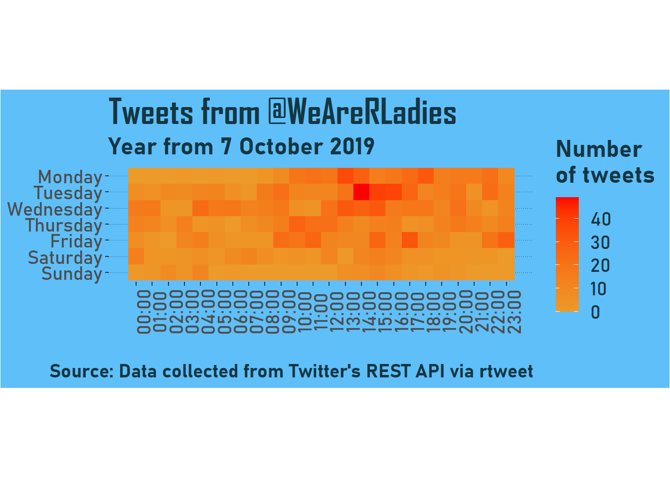 Things look busiest on weekdays, as shown before, particularly around the early afternoon. Tuesday afternoon is the busiest patch - perhaps when people are getting stuck into their biggest planned piece for the curation!
Also, these times are in UTC, based on me being in the UK. It makes sense to me that the afternoon is busy, therefore, because @WeAreRLadies is a global account. Early to mid afternoon captures curators in the Americas tweeting first thing in the morning, people in Europe and Africa tweeting in the afternoon and for some places in Asia will include tweets later in the day. So it’s probably the biggest crossover period for a lot of curators across the world.
I’m going to post one more time on tweets from this account - next time I’ll be looking at hashtags.